Interpolation between grids with Basemap

Task:

Interpolate data from regular to curvilinear grid

Solution:

Basemap.interp function

Unfortunately geophysical data distributed on a large variety of grids, and from time to time we have to compare our variables to each other. Often plotting a simple map is enough, but if you want to go a bit beyond qualitative comparison then you have to interpolate data from one grid to another. One of the easiest way to do this is to use basemap.interp function from Matplotlib Basemap library. Here I will show how to prepare your data and how to perform interpolation.

Some necessary imports:

In [ ]:
%pylab inline
In [ ]:
from scipy.io import netcdf

As usual we are going to use NCEP reanalysis data. This time monthly mean air temperature. Load with wget:

In [ ]:
!wget ftp://ftp.cdc.noaa.gov/Datasets/ncep.reanalysis.derived/surface/air.mon.mean.nc

We also need coordinates of the curvilinear grid:

In [ ]:
!wget https://www.dropbox.com/s/9xzgyjs08zyuwzw/curv_grid.nc

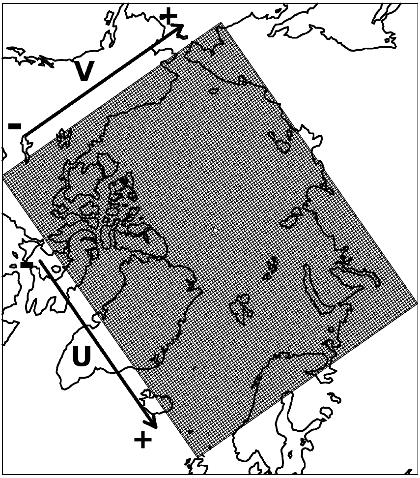
Let's have a look at our curvilinear grid:

In [30]:
fc = netcdf.netcdf_file('curv_grid.nc')
lon_curv = fc.variables['xc'][0,:,:]
lat_curv = fc.variables['yc'][0,:,:]

Distribution of longitudes, for example, looks like this:

In [31]:
imshow(lon_curv)
Out[31]:

This is grid from the regional Arctic Ocean model with 40 km resolution:

Now load NCEP data (only first time step), that have 2.5 degree resolution:

In [32]:
fr = netcdf.netcdf_file('air.mon.mean.nc')
In [33]:
air = fr.variables['air'][0,:,:]
lat = fr.variables['lat'][:]
lon = fr.variables['lon'][:]

First look at the data:

In [34]:
imshow(air)
#colorbar()
Out[34]:

and longitudes (1d):

In [35]:
lon
Out[35]:
array([   0. ,    2.5,    5. ,    7.5,   10. ,   12.5,   15. ,   17.5,
         20. ,   22.5,   25. ,   27.5,   30. ,   32.5,   35. ,   37.5,
         40. ,   42.5,   45. ,   47.5,   50. ,   52.5,   55. ,   57.5,
         60. ,   62.5,   65. ,   67.5,   70. ,   72.5,   75. ,   77.5,
         80. ,   82.5,   85. ,   87.5,   90. ,   92.5,   95. ,   97.5,
        100. ,  102.5,  105. ,  107.5,  110. ,  112.5,  115. ,  117.5,
        120. ,  122.5,  125. ,  127.5,  130. ,  132.5,  135. ,  137.5,
        140. ,  142.5,  145. ,  147.5,  150. ,  152.5,  155. ,  157.5,
        160. ,  162.5,  165. ,  167.5,  170. ,  172.5,  175. ,  177.5,
        180. ,  182.5,  185. ,  187.5,  190. ,  192.5,  195. ,  197.5,
        200. ,  202.5,  205. ,  207.5,  210. ,  212.5,  215. ,  217.5,
        220. ,  222.5,  225. ,  227.5,  230. ,  232.5,  235. ,  237.5,
        240. ,  242.5,  245. ,  247.5,  250. ,  252.5,  255. ,  257.5,
        260. ,  262.5,  265. ,  267.5,  270. ,  272.5,  275. ,  277.5,
        280. ,  282.5,  285. ,  287.5,  290. ,  292.5,  295. ,  297.5,
        300. ,  302.5,  305. ,  307.5,  310. ,  312.5,  315. ,  317.5,
        320. ,  322.5,  325. ,  327.5,  330. ,  332.5,  335. ,  337.5,
        340. ,  342.5,  345. ,  347.5,  350. ,  352.5,  355. ,  357.5], dtype=float32)

There are couple of problems with this longitude. First - Basemap wants it to be in the -180:180 format, not 0:360. This can be fixed:

In [36]:
lon1 = lon.copy()
for n, l in enumerate(lon1):
    if l >= 180:
       lon1[n]=lon1[n]-360. 
lon = lon1
In [37]:
lon
Out[37]:
array([   0. ,    2.5,    5. ,    7.5,   10. ,   12.5,   15. ,   17.5,
         20. ,   22.5,   25. ,   27.5,   30. ,   32.5,   35. ,   37.5,
         40. ,   42.5,   45. ,   47.5,   50. ,   52.5,   55. ,   57.5,
         60. ,   62.5,   65. ,   67.5,   70. ,   72.5,   75. ,   77.5,
         80. ,   82.5,   85. ,   87.5,   90. ,   92.5,   95. ,   97.5,
        100. ,  102.5,  105. ,  107.5,  110. ,  112.5,  115. ,  117.5,
        120. ,  122.5,  125. ,  127.5,  130. ,  132.5,  135. ,  137.5,
        140. ,  142.5,  145. ,  147.5,  150. ,  152.5,  155. ,  157.5,
        160. ,  162.5,  165. ,  167.5,  170. ,  172.5,  175. ,  177.5,
       -180. , -177.5, -175. , -172.5, -170. , -167.5, -165. , -162.5,
       -160. , -157.5, -155. , -152.5, -150. , -147.5, -145. , -142.5,
       -140. , -137.5, -135. , -132.5, -130. , -127.5, -125. , -122.5,
       -120. , -117.5, -115. , -112.5, -110. , -107.5, -105. , -102.5,
       -100. ,  -97.5,  -95. ,  -92.5,  -90. ,  -87.5,  -85. ,  -82.5,
        -80. ,  -77.5,  -75. ,  -72.5,  -70. ,  -67.5,  -65. ,  -62.5,
        -60. ,  -57.5,  -55. ,  -52.5,  -50. ,  -47.5,  -45. ,  -42.5,
        -40. ,  -37.5,  -35. ,  -32.5,  -30. ,  -27.5,  -25. ,  -22.5,
        -20. ,  -17.5,  -15. ,  -12.5,  -10. ,   -7.5,   -5. ,   -2.5], dtype=float32)

Second - the order of both lat and lon should be increasing. So we have to reshape our longitudes and data in a way that the first values on the left correspond to -180 longitude. We split arrays in the middle:

In [38]:
air1 = air[:,0:72]
air2 = air[:,72:]
lon1 = lon[0:72]
lon2 = lon[72:]

And then put this halves back together, but switching left and right:

In [39]:
air_new = np.hstack((air2, air1))
lon_new = np.hstack((lon2, lon1))

Now lons look OK:

In [40]:
lon_new
Out[40]:
array([-180. , -177.5, -175. , -172.5, -170. , -167.5, -165. , -162.5,
       -160. , -157.5, -155. , -152.5, -150. , -147.5, -145. , -142.5,
       -140. , -137.5, -135. , -132.5, -130. , -127.5, -125. , -122.5,
       -120. , -117.5, -115. , -112.5, -110. , -107.5, -105. , -102.5,
       -100. ,  -97.5,  -95. ,  -92.5,  -90. ,  -87.5,  -85. ,  -82.5,
        -80. ,  -77.5,  -75. ,  -72.5,  -70. ,  -67.5,  -65. ,  -62.5,
        -60. ,  -57.5,  -55. ,  -52.5,  -50. ,  -47.5,  -45. ,  -42.5,
        -40. ,  -37.5,  -35. ,  -32.5,  -30. ,  -27.5,  -25. ,  -22.5,
        -20. ,  -17.5,  -15. ,  -12.5,  -10. ,   -7.5,   -5. ,   -2.5,
          0. ,    2.5,    5. ,    7.5,   10. ,   12.5,   15. ,   17.5,
         20. ,   22.5,   25. ,   27.5,   30. ,   32.5,   35. ,   37.5,
         40. ,   42.5,   45. ,   47.5,   50. ,   52.5,   55. ,   57.5,
         60. ,   62.5,   65. ,   67.5,   70. ,   72.5,   75. ,   77.5,
         80. ,   82.5,   85. ,   87.5,   90. ,   92.5,   95. ,   97.5,
        100. ,  102.5,  105. ,  107.5,  110. ,  112.5,  115. ,  117.5,
        120. ,  122.5,  125. ,  127.5,  130. ,  132.5,  135. ,  137.5,
        140. ,  142.5,  145. ,  147.5,  150. ,  152.5,  155. ,  157.5,
        160. ,  162.5,  165. ,  167.5,  170. ,  172.5,  175. ,  177.5], dtype=float32)

And this is our new data array:

In [41]:
imshow(air_new)
Out[41]:

What about lats?

In [42]:
lat
Out[42]:
array([ 90. ,  87.5,  85. ,  82.5,  80. ,  77.5,  75. ,  72.5,  70. ,
        67.5,  65. ,  62.5,  60. ,  57.5,  55. ,  52.5,  50. ,  47.5,
        45. ,  42.5,  40. ,  37.5,  35. ,  32.5,  30. ,  27.5,  25. ,
        22.5,  20. ,  17.5,  15. ,  12.5,  10. ,   7.5,   5. ,   2.5,
         0. ,  -2.5,  -5. ,  -7.5, -10. , -12.5, -15. , -17.5, -20. ,
       -22.5, -25. , -27.5, -30. , -32.5, -35. , -37.5, -40. , -42.5,
       -45. , -47.5, -50. , -52.5, -55. , -57.5, -60. , -62.5, -65. ,
       -67.5, -70. , -72.5, -75. , -77.5, -80. , -82.5, -85. , -87.5, -90. ], dtype=float32)

They are not increasing, and we have to flip them up side down:

In [43]:
lat_new = np.flipud(lat)
lat_new
Out[43]:
array([-90. , -87.5, -85. , -82.5, -80. , -77.5, -75. , -72.5, -70. ,
       -67.5, -65. , -62.5, -60. , -57.5, -55. , -52.5, -50. , -47.5,
       -45. , -42.5, -40. , -37.5, -35. , -32.5, -30. , -27.5, -25. ,
       -22.5, -20. , -17.5, -15. , -12.5, -10. ,  -7.5,  -5. ,  -2.5,
         0. ,   2.5,   5. ,   7.5,  10. ,  12.5,  15. ,  17.5,  20. ,
        22.5,  25. ,  27.5,  30. ,  32.5,  35. ,  37.5,  40. ,  42.5,
        45. ,  47.5,  50. ,  52.5,  55. ,  57.5,  60. ,  62.5,  65. ,
        67.5,  70. ,  72.5,  75. ,  77.5,  80. ,  82.5,  85. ,  87.5,  90. ], dtype=float32)

The data should be flipped accordingly:

In [44]:
air_new = np.flipud(air_new)

Now import mpl_toolkits.basemap:

In [45]:
import  mpl_toolkits.basemap  

and interpolate:

In [46]:
result = mpl_toolkits.basemap.interp(air_new, lon_new, lat_new, \
                                     lon_curv, lat_curv, checkbounds=False, masked=False, order=1)

Here as an input we use our modified 1d coordinate variables and data, as well as two 2d arrays with coordinates of curvilinear grid we interpolate to. You can change type of interpolation by setting the order argument. It is 0 for nearest-neighbor interpolation, 1 for bilinear interpolation, 3 for cubic spline (default 1).

Quick look at the result:

In [47]:
imshow(result)
colorbar()
Out[47]:

Not very clear what we get here. Let's put this data on the map:

In [48]:
from mpl_toolkits.basemap import Basemap
In [49]:
m = Basemap(projection='npstere',boundinglat=40,lon_0=0,resolution='l')
x, y = m(lon_curv, lat_curv)
lon_new2, lat_new2 = meshgrid(lon_new, lat_new)
x2, y2 = m(lon_new2, lat_new2)
In [50]:
fig = plt.figure(figsize=(10,10))
subplot(121)
m.drawcoastlines(linewidth=1.)
cs = m.contourf(x,y,result, levels = np.arange(-40,10,5), extend='both')
colorbar(orientation='horizontal')

subplot(122)
m.drawcoastlines(linewidth=1.)
cs = m.contourf(x2,y2,air_new, levels = np.arange(-40,10,5), extend='both')
colorbar(orientation='horizontal')
Out[50]:

Look quite similar to me :)

But if we look at pcolor versions of figures, were grid is visible, you will see what basemap.interp did.

In [51]:
fig = plt.figure(figsize=(10,20))
subplot(211)
m.drawcoastlines(linewidth=1.)
cs = m.pcolormesh(x,y,result, vmin =-40, vmax=10)

subplot(212)
m.drawcoastlines(linewidth=1.)
cs = m.pcolormesh(x2,y2,air_new, vmin =-40, vmax=10)

Comments !

links

social